A schematic impression of the binary pulsar PSR1913+16, which was the first indirect detection of gravitational waves and relied on an O-C diagram. (Credit: Nobel Media)

Observed-minus-calculated (O-C) diagrams are an extremely powerful tool that allows us to witness very subtle changes in periodic astrophysical phenomena. These diagrams have been instrumental in our quest to observe the influence of gravitational radiation, in systems with binary pulsars as well as binary white dwarfs. These diagrams compare the timing of an event (say the mid-point of an eclipse or the peak of a pulsation cycle) to when we expect such an event if it occurred at an exactly constant periodicity. It may help to visualize an example:

Imagine a leaky faucet that keeps exceptionally precise time, left unattended for many decades. Its drip rate is very slow -- every 12 minutes a drop of water falls to a basin below, and we can measure the time these drips hit the basic with good precision, to better than a little less than a second.

Now imagine the water isn't perfectly pure, and these impurities build up as sediment slowly but in a constant way. This sediment very slowly lengthens the period between drips, causing them to occur less and less frequently. In this case, let's imagine the buildup is incredibly gradual, and that the original drip period of exactly 12 minutes is changing by just 0.5 milliseconds every year (0.5 ms/yr).

By building an (O-C) diagram we can measure such a sub-millisecond change in the drip period over a year, even if we can only measure each drip to an accuracy of about 1 second. Our leverage comes from the first observation, and the fact that the deviation in later observations compared to our first observation piles up the longer we observe our leaky sink. This change from the original observations --- what we observe (O) versus what we calculate (C) given a perfectly constant period -- is at the heart of the (O-C) diagram.

For simplicity sake, let's say that we measured a drip to occur at exactly midnight on 1 January 2014, at UT 00:00:00 (the UTC midnight on 1 Jan 2014 corresponds to a Julian date of 2456658.5, which is a natural unit of absolute time for astronomers). We observe a drip around midnight on the first of every month and record the absolute time that drip hit the basin. If there were no sediment buildup, the time of the drip would be perfectly constant, always separated by exactly 12 minutes. After a year, the 43800th drip would occur exactly at midnight on 1 January 2015. Instead, we have stated that the drip period is increasing by half a millisecond every year.

It's natural to expect that when we go and look on 1 January 2015 we'd see a drip occur 0.5 ms after midnight. Instead, we would measure that drip to occur at about UT 00:00:11 on 1 January 2015; the drip would occur nearly 11 s after midnight! Sure enough, the time between drips has only changed by half a millisecond in the year between 1 January 2014 and 1 January 2015, so that the period after one year would be P = 12.00000833 min (720.0005 s). But the drip itself would be delayed by more than 10 s.

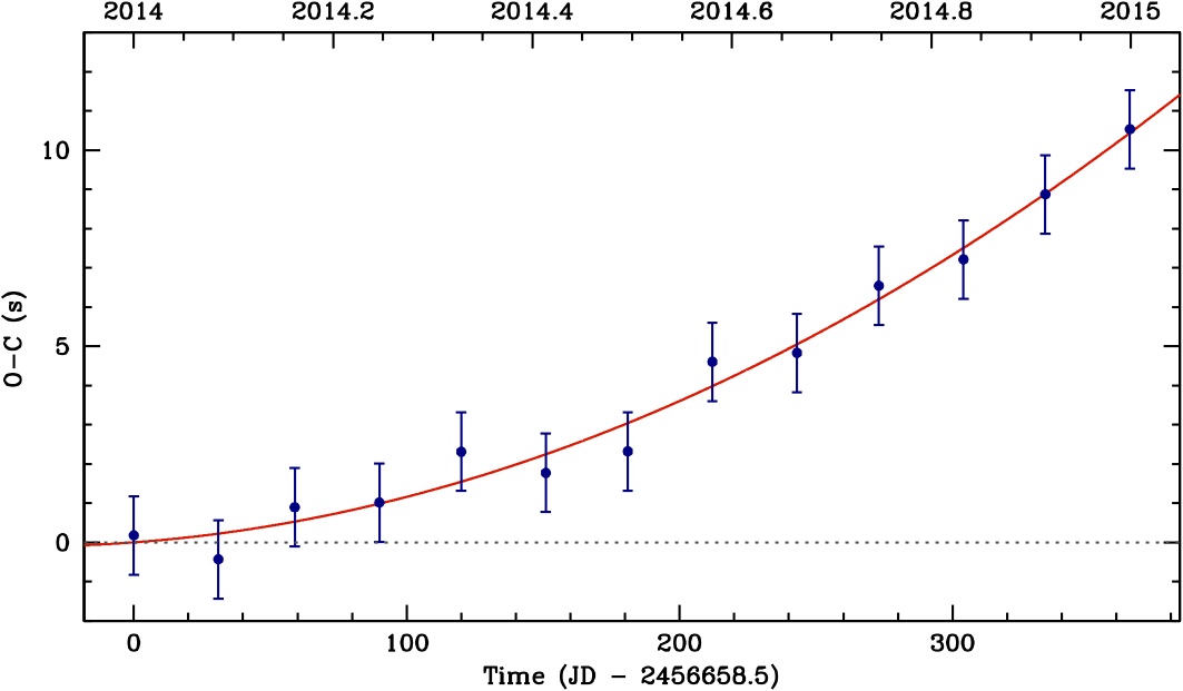
An (O-C) diagram for our thought experiment of a leaky faucet that keeps excellent time but which has a drip period that is lengthening slightly, by 0.5 ms each year from an initial drip period of 12 minutes. Our first observation occurred exactly at midnight on 1 Jan 2014, and we subsequently show here how much time has elapsed after midnight before we observed a drip on the first of every month. The best-fit red parabola to the observations measures the rate of period change.

The above figure illustrates this thought experiment, showing the (O-C) diagram of when we observe the drips versus when we'd expect them given an exactly constant drip period. The grey dotted line shows the line of (O-C) = 0 s; what we would "expect" for a perfectly constant period. Our "observations" are shown in dark blue and have been perturbed by random Gaussian noise assuming 1 s uncertainties for each observation. These "observations" essentially correspond to how much time after midnight we observe the drip at the beginning of each month.

Even though the period change is quite slow (0.5 ms/yr), and we can only measure the time of a drip to about 1 s accuracy, we would have a nearly 3-sigma measurement of the rate of drip period change, accurate to a fraction of a millisecond per year, after just 13 measurements over one year of monitoring! In our example, we would be able to measure a rate of period change of dP/dt = (1.24 ± 0.47) × 10^-11 s/s (or 0.39 ± 0.15 ms/yr) from the red best-fit parabola in the figure above. This thought experiment illustrates the power of constructing a long-term (O-C) diagram in measuring very small rates of period change.

It may help to fully derive the formula for these drip changes. Following Kepler et al. (1991), if the drip period is changing slowly with time, we can expand the observed time of the Eth drip, t_E, in a Taylor series around E_0:

where the epoch is E=t/P and the change in arrival time with epoch, dt/dE, is simply the period, P. If we drop all terms higher than second order (assuming that the period acceleration is negligible), we arrive at the classic (O-C) equation:

where t_0 is the time of the first drip, Δt_0 is the uncertainty in this time, P_0 is the drip period at this time of first drip and ΔP_0 is the error in the observed period. Thus, any secular change in the period, dP/dt, will cause a parabolic curvature in an (O-C) diagram (a bad period with cause the ΔP_0 term to dominate and the (O-C) will be a straight line). Hence, the key is that the effect piles up with time squared, as we can finally write this (O-C) formula in terms of the time of observations: